Introduction
- Visualizes high-dimensional data by giving each data point a location in a 2 or 3-dimensional map.
- Most of these techniques simply provide tools to display more than two data dimensions, and leave the interpretation of the data to the human observer.
- The aim of dimensionality reduction is to preserve as much of the significant structure of the high-dimensional data as possible in the low-dimensional map.
- 传统的线性技术主要是想让不相似的点在低维表示中分开。
- PCA(Principle Components Analysis,主成分分析)
- MDS(Multiple Dimensional Scaling,多维缩放)
- 对于处于低维、非线性流形上的高维数据而言,更重要的是让相似的近邻点在低维表示中靠近。非线性技术主要保持数据的局部结构。
- Sammon mapping
- CCA(Curvilinear Components Analysis)
- SNE(Stochastic Neighbor Embedding,随机近邻嵌入),t-SNE是基于SNE的。
- Isomap(Isometric Mapping,等度量映射)
- MVU(Maximum Variance Unfolding)
- LLE(Locally Linear Embedding,局部线性嵌入)
- Laplacian Eigenmaps
- In particular, most of the techniques are not capable of retaining both the local and the global structure of the data in a single map.
- In this paper, we introduce
- a way of converting a high-dimensional data set into a matrix of pairwise similarities and,
- a new technique, called “t-SNE”, for visualizing the resulting similarity data.
SNE
Stochastic Neighbor Embedding,随机近邻嵌入
SNE starts by converting the high-dimensional Euclidean distances between datapoints into conditional probabilities that represent similarities.
- 一种基于概率的数据降维处理方法。
- 可以提供原始数据,也可以只提供点之间的相似度,两种输入均可。
Given a set of high-dimensional data points \(x_1, x_2, ..., x_n\), \(p_{i|j}\) is the conditional probability that \(x_i\) would pick \(x_j\) as its neighbor if neighbors were picked in proportion to their probability density under a Gaussian centered at \(x_i\).
\[p_{j|i} = \frac{exp(-||x_i-x_j||^2/2\sigma_i^2)}{\sum_{k\neq i}exp(-||x_i-x_k||^2/2\sigma_i^2)}\]
注意:1)分母即归一化。2)默认\(p_{i|i}=0\)。3)每不同数据点\(x_i\)有不同的\(\sigma_i\)。其计算方式下面说。
Similarly, define \(q_{i|j}\) as conditional probability corresponding to low-dimensional representations of \(y_i\) and \(y_j\) (corresponding to \(x_i\) and \(x_j\)). The variance of Gaussian in this case is set to be \(1/\sqrt{2}\).
\[q_{j|i} = \frac{exp(-||y_i-y_j||^2)}{\sum_{k\neq i}exp(-||y_i-y_k||^2)}\]
注意:1)\(\sigma_i\) 若取其他值,对结果影响仅仅是缩放而已。
If the map points \(y_i\) and \(y_j\) correctly model the similarity between the high-dimensional data points \(x_i\) and \(x_j\), the conditional probabilities \(p_{j|i}\) and \(q_{j|i}\) will be equal.
SNE aims to find a low-dimensional data representation that minimizes the mismatch between \(p_{j|i}\) and \(q_{j|i}\). Thus we use the sum of Kullback-Leibler divergences over all data points as the cost function:
\[C=\sum_i KL(P_i||Q_i) = \sum_i \sum_j p_{j|i} log\frac{p_{j|i}}{q_{j|i}}\]
in which \(P_i(k=j)=p_{j|i}\) represents the conditional probability distribution over all other data points given data point \(x_i\). \(Q_i(k=j)=q_{j|i}\) too.
注意:KLD是不对称的!因为 \(KLD=p log(\frac{p}{q})\),p>q时为正,p<q时为负。则如果高维数据相邻而低维数据分开(即p大q小),则cost很大;相反,如果高维数据分开而低维数据相邻(即p小q大),则cost很小。所以SNE倾向于保留高维数据的局部结构。
对\(C\)进行梯度下降即可以学习到合适的\(y_i\)。
The gradient:
\[\frac{\partial C}{\partial y_i} = 2 \sum_j (p_{j|i} - q_{j|i} + p_{i|j} - q_{i|j})(y_i - y_j)\]
and the gradient update with a momentum term:(这里给出但个\(y_i\)点的梯度下降公式,显然需要对所有\(\mathcal{Y}^{(T)}=\{y_1, y_2, ..., y_n\}\)进行统一迭代。)
\[y_i^{(t)} = y_i^{(t-1)} + \eta \frac{\partial C}{\partial y_i} + \alpha(t)( y_i^{(t-1)} - y_i^{(t-2)})\]
t-SNE has a cost function that is not convex, i.e. with different initializations we can get different results. 很难优化,也对初值十分敏感,因此要跑多次SNE选取KLD最小/可视化最好结果。(注意这个不是为了泛化,因此选最好的结果即可。)
如何为每一个\(x_i\)选取对应的\(\sigma_i\)?
It is not likely that there is a single value of \(\sigma_i\) that is optimal for all data points in the data set because the density of the data is likely to vary. In dense regions, small \(\sigma_i\), while in sparse region, large \(\sigma_i\).
Every \(\sigma_i\) is either set by hand (不忍吐槽,原话见于(Hinton and Roweis, 2003)) or found by a simple binary search (Hinton and Roweis, 2003) or by a very robust root-finding method (Vladymyrov and Carreira-Perpinan, 2013)
使用算法来确定\(\sigma_i\)要求用户预设困惑度(perplexity)。然后算法找到合适的\(\sigma_i\)值让条件分布\(P_i\)的困惑度等于用户预定义的困惑度即可。
\[Perp(P_i) = 2^{H(P_i)} = 2^{-\sum_j p_{j|i} log_2 p_{j|i}}\]
注意:困惑度设的大,则显然\(\sigma_i\)也大。The perplexity increases monotonically with the variance \(\sigma_i\).
The perplexity can be interpreted as a smooth measure of the effective number of neighbors. The performance of SNE is fairly robust to changes in the perplexity, and typical values are between 5 and 50.
t-SNE
- t-Distributed Stochastic Neighbor Embedding
- SNE有两个问题:
- Cost function 难以优化 -> 解决方案:使用Symmetric SNE。
- Crowding Problem -> 解决方案:在低维嵌入上使用Student’s t-distribution替代Guassian distribution,同时也简化了cost function。
Symmetric SNE
We define the joint probabilities \(p_{ij}\) in the high-dimensional space to be the symmetrized conditional probabilities, that is, we set
\[p_{ij} = \frac{p_{j|i} + p_{i|j}}{2n}\]
minimizing the sum of KLD between conditional probabilities -> minimizing a single KLD between joint probability distribution.
\[C = KL(P||Q) = \sum_i \sum_j p_{ij} log \frac{p_{ij}}{q_{ij}}\]
The main advantage of the symmetric version of SNE is the simpler form of its gradient, which is faster to compute.
\[\frac{\partial C}{\partial y_i} = 4 \sum_j (p_{ij} - q_{ij})(y_i - y_j)\]
(注意:这只是Symmetric SNE的梯度公式,t-SNE的梯度公式类似,推导见后。)
Crowding Problem
“crowding problem”: the area of the two-dimensional map that is available to accommodate moderately distant datapoints will not be nearly large enough compared with the area available to accommodate nearby datapoints.
这句话的意思是:在二维映射空间中,能容纳(高维空间中的)中等距离间隔点的空间,不会比能容纳(高维空间中的)相近点的空间大太多。 换言之,哪怕高维空间中离得较远的点,在低维空间中留不出这么多空间来映射。于是到最后高维空间中远的、近的点,在低维空间中统统被塞在了一起,这就叫做“拥挤问题(Crowding Problem)”。
Note that the crowding problem is not specific to SNE, but that it also occurs in other local techniques for multidimensional scaling such as Sammon mapping.
One way around this problem is to use UNI-SNE (Cook et al. 2007)
这种方法直接给低维空间的点给予一个均匀分布(uniform dist),使得对于高维空间中距离较远的点(\(p_{ij}\)较小),强制保证在低维空间中\(q_{ij}>p_{ij}\) (因为均匀分布的两边比高斯分布的两边高出太多了)。
Although UNI-SNE usually outperforms standard SNE, the optimization of the UNI-SNE cost function is tedious.
在低维空间中使用均匀分布(UNI-SNE)替代高斯分布(SNE),但cost function优化很复杂,这也是转而使用t分布(t-SNE)取代高斯分布(SNE)的动机。
t-SNE
Instead of Gaussian, use a heavy-tailed distribution (like Student-t distribution) to convert distances into probability scores in low dimensions. This way moderate distance in high-dimensional space can be modeled by larger distance in low-dimensional space.
Student’s t-distribution
Student’s t-distribution has the probability density function given by
\[f(t) = \frac{\Gamma(\frac{\nu + 1}{2})}{\sqrt{\nu \pi}\Gamma(\frac{\nu}{2})}(1 + \frac{t^2}{\nu})^{-\frac{\nu + 1}{2}}\]
where \(\nu\) is the number of degrees of freedom.
Special cases \(\nu = 1\)
\[f(t) = \frac{1}{\pi (1+t^2)}\]
Called Cauchy distribution. 我们用到是这个简单形式。
Special cases \(\nu = \infty\)
\[f(t) = \frac{1}{\sqrt{2\pi}} e^{-\frac{t^2}{2}}\]
Called Guassian/Normal distribution.
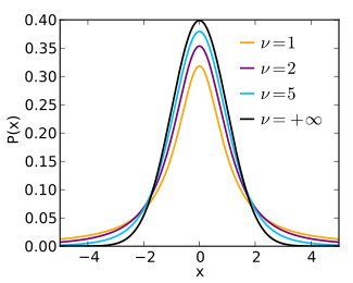
figure of probability density function
Why choose t-dist?
- it is closely related to the Gaussian distribution, as the Student t-distribution is an infinite mixture of Gaussians.
- A computationally convenient property is that it is much faster to evaluate the density of a point under a Student t-distribution than under a Gaussian because it does not involve an exponential.
Why choose t-dist with single degree of freedom?
Because it has particularly nice property: inverse square law. This makes the map’s representation of joint probabilities (almost) invariant to changes in the scale of the map for map points that are far apart. 意思是:这个平方反比的形式,使得当高维空间的两个点再远,他们在低维空间的联合概率几乎不变。结合上一节提到的UNI-SNE:
给低维空间的点给予一个均匀分布(uniform dist),使得对于高维空间中距离较远的点(\(p_{ij}\)较小),强制保证在低维空间中\(q_{ij}>p_{ij}\) (因为均匀分布的两边比高斯分布的两边高出太多了)。
从上面的t分布图中可以看到,由于t分布的尾巴高于高斯分布的尾巴,使用t分布同样可以保证对于高维空间中的远距离点,使得在低维空间中\(q_{ij}>p_{ij}\)。
The joint probabilities \(q_{ij}\) are defined as
\[q_{ij} = \frac{(1 + ||y_i - y_j||^2)^{-1}}{\sum_{k\neq l}(1+||y_k - y_l||^2)^{-1}}\]
(注意:和SNE的\(q_{j|i}\)公式相比,分母中求和号中,之前是\(k\neq i\),表示仅排除\(i\)自身项;现在是\(k\neq l\),表示排除所有自身项 )
The cost function is easy to optimize.
\[\frac{\partial C}{\partial y_i} = 4 \sum_j (p_{ij} - q_{ij})(y_i - y_j)(1+ ||y_i - y_j||^2)^{-1}\]
(注意:是在Symmetric SNE的梯度公式后面加上了\((1+ ||y_i - y_j||^2)^{-1}\)一项,推导见论文附录A。)
Complexity
- Space and time complexity is quadratic (\(O(n^2)\)) in the number of datapoints so infeasible to apply on large datasets.
- Random walk
- Select a random subset of points (called landmark points) to display.
- for each landmark point, define a random walk starting at a landmark point and terminating at any other landmark point.
- \(p_{i|j}\) is defined as fraction of random walks starting at \(x_i\) and finishing at \(x_j\) (both these points are landmark points). This way, \(p_{i|j}\) is not sensitive to “short-circuits” in the graph (due to noisy data points).
- Barnes-Hut approximations (Van Der Maaten, 2014)
- allowing it to be applied on large real-world datasets. We applied it on data sets with up to 30 million examples.
Advantages of t-SNE
- Gaussian kernel employed by t-SNE (in high-dimensional) defines a soft border between the local and global structure of the data.
- Both nearby and distant pair of datapoints get equal importance in modeling the low-dimensional coordinates.
- The local neighborhood size of each datapoint is determined on the basis of the local density of the data.
- Random walk version of t-SNE takes care of “short-circuit” problem.
Limitations of t-SNE
- it is unclear how t-SNE performs on general dimensionality reduction tasks,
- the relatively local nature of t-SNE makes it sensitive to the curse of the intrinsic dimensionality of the data, and
- t-SNE is not guaranteed to converge to a global optimum of its cost function.
彩蛋
关于SNE的梯度公式
\[\frac{\partial C}{\partial y_i} = 2 \sum_j (p_{j|i} - q_{j|i} + p_{i|j} - q_{i|j})(y_i - y_j)\]
作者在论文第4页用了一个弹簧的比喻来解释,如图:
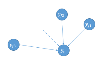
spring
可以把该公式看做是所有\(y_j\)通过弹簧(图中箭头)对\(y_i\)的合力,类比胡克定律\(F=k\Delta x\),这里\((y_i - y_j)\)表示拉伸长度,而\((p_{j|i} - q_{j|i} + p_{i|j} - q_{i|j})\)表示弹性系数。表示高维数据点和低维映射点之间点相似度的失配程度(mismatch between the pairwise similarities of the data points and the map points)。按这么来说,弹性系数应该写成\((\frac{p_{j|i} + p_{i|j}}{2} - \frac{q_{j|i} + q_{i|j}}{2})\)的形式,有趣的是,如果写成这种形式,则SNE、Symmetric SNE、t-SNE的梯度公式形式上就统一了。
- SNE: \[\frac{\partial C}{\partial y_i} = 4 \sum_j (\frac{p_{j|i} + p_{i|j}}{2} - \frac{q_{j|i} + q_{i|j}}{2})(y_i - y_j)\]
- Symmetric SNE: \[\frac{\partial C}{\partial y_i} = 4 \sum_j (p_{ij} - q_{ij})(y_i - y_j)\]
- t-SNE: \[\frac{\partial C}{\partial y_i} = 4 \sum_j (p_{ij} - q_{ij})(y_i - y_j)(1+ ||y_i - y_j||^2)^{-1}\]