本文是哈工大2017年秋季《数据挖掘理论与算法》课程实验第一大题的实验报告。
主要实现了Apriori算法和FP-Growth算法并对他们做了时间、内存性能上的比较。
实验说明书和源代码参见GitHub Repo。实验要求也可以见于每一小节的开头。
Algorithm Implementation
(a) Describe your implementation. If open-source software is referenced, please acknowledge the authors of the software.
In this project we use Python to implement two different frequent itemset mining algorithms Apriori and FP-Growth. The basic principle of two algorithms are already introduced in the class. Therefore, we just introduce the basic steps here.
Machine Learning in Action is the only reference source. We didn’t copy the code but write it again to make them more clear and understandable.
Hardware/Software Configuration
- Hardware
- CPU: Intel(R) Xeon(R) CPU E5-2678 v3 @ 2.50GHz
- Core Number: 48
- Memory: 60G
- Software
- Ubuntu 14.04 LTS
- Python 3.5
Apriori
Apriori Principle: The non-empty subsets of a frequent itemset is frequent, which means, the supersets of a infrequent itemset is also infrequent.
- Candidate generate
- Candidate pruning
The framework / basic APIs of the code is as below, I do the comment to explain the usage of each method. To see the complete code please refer to the appendix.
|
|
FP Growth
FP Growth algorithm applies the Apriori Principle too, instead, it build a FP Tree in the beginning. This data structure helps it to mine the frequent itemsets more effectively.
- Build the FP tree and the header table.
- Recursively generate the conditional pattern bases.
- Mining the tree
The framework / basic APIs of the code is as below, I do the comment to explain the usage of each method. To see the complete code please refer to the appendix.
|
|
Verification
We construct a toy transaction dataset to verify whether the programs are implemented correctly. The toy dataset is derived from the handout given by Prof. Zou in class.
The result of Apriori algorithm is as below:
|
|
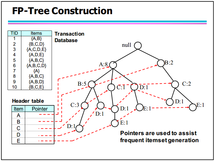
The result of FP Growth algorithm is as below: (with a visualized FP Tree)
|
|
The results indicate the correctness of our implementation.
Parallel Programming
Since this experiment requires lots of results to observe the impact of several parameters, running the programs one by one may looks clumsy and wastes lots of time. We run our algorithm on a multi-CPU server in parallel. On this point we use a Pythonic way to run our programs in parallel automatically.
In Python,we can uses a class named multiprocessing.Pool to run multiple command on multiple CPU cores in parallel.
|
|
We need to write all bash commands (like python apriori.py with different parameters) in cmd_list (in form of strings). Instance pool will assign each task to a core then os.system will execute each command. In this way, we can run 48 experiment at the same time and save lots of time!
Datasets Generation
(b) Generate synthetic datasets using the IBM Synthetic Data Generator for Itemsets and Sequences available at https://github.com/zakimjz/IBMGenerator.
In order to fine-tune the parameters we need a more complicated dataset generator rather than some toy datasets. We use the IBM Synthetic Data Generator to generate the Itemsets.
Use the bash commands below to download and compile the tool.
|
|
Use the bash commands below to generate a toy dataset.
|
|
Where -ntrans controls the number of transactions, -tlen controls the length of transactions, -nitems controls the number of distinct items. These three arguments are important to us since we need to fine tune them to observe the performance of the algorithms.
Use the bash commands below to view the dataset.
|
|
The 1st column is CustID, 2nd column is TransID, 3rd column is NumItems and the rests are Items. (We only use the Items data.)
Here we encapsulate this data generator into a Python function, which generate the IBM format data and convert to the data that Python can read, like this:
|
|
Parameters Fine-tuning
(c) Test the impact of the following parameters on the performance (e.g., running time and memory comsumption) of the algorithms.
• The minimum support threshold minsup
• The number of transactions
• The length of transactions
• The number of distinct items
In this Chapter we will use IBM Synthetic Data Generator and the algorithms we implemented, to fine-tune 4 kinds of parameters as required in the
Tools & Evaluation Metrics
In order to collect the information of time and memory consumed by the algorithms, we introduce a Pythonic way to measure them. we use two powerful tools line_profiler and memory_profiler. In order to install them, just type
|
|
Then insert decorator @profile before the methods we interest in in the code, like this
|
|
Then run your code in this way if you want to observe the consumed time:
|
|
… and in this way if you want to observe the consumed memory:
|
|
In this way we can observe the consumed time and memory line by line. We will soon use this tool to collect the data we need.
☆☆☆ Notice that: Using the line_profiler and memory_profiler will increase the total running time (roughly x1 to x5). The more decorator @profile you add before methods, the slower the program.
Experiment Design
The parameters we set are as follows:
- Default:
ntrans=5(k), tlen=10, nitems=1(k), minsup=0.02
Fine-tune one of the parameter and keep other 3 default. The fine-tuned parameters are set as follows:
- number of transactions(
ntrans):
[1, 2, 3, 4, 5, 6, 7, 8, 9, 10, 11, 12, 13, 14, 15, 16, 17, 18, 19, 20] (Unit: k)
- length of transaction(
tlen):
[1, 2, 3, 4, 5, 6, 7, 8, 9, 10, 11, 12, 13, 14, 15, 16, 17, 18, 19, 20]
- number of items(
nitems):
[0.1, 0.2, 0.3, 0.4, 0.5, 0.6, 0.7, 0.8, 0.9, 1.0, 1.1, 1.2, 1.3, 1.4, 1.5, 1.6, 1.7, 1.8, 1.9, 2.0] (Unit: k)
- minimal support threshold(
minsup):
[0.01, 0.02, 0.03, 0.04, 0.05, 0.06, 0.07, 0.08, 0.09, 0.1, 0.11, 0.12, 0.13, 0.14, 0.15, 0.16, 0.17, 0.18 , 0.19, 0.2]
In this way, we derive 20x4=80 results. We draw four line charts for each fine-tuned parameter as follows:
Time Performance
Notice that:
- The red full line represents Apriori, the blue dash line represents FP Growth.
- The real time should divide by roughly 3, since the
line_profilerwill make the program slower roughly x1~x5.
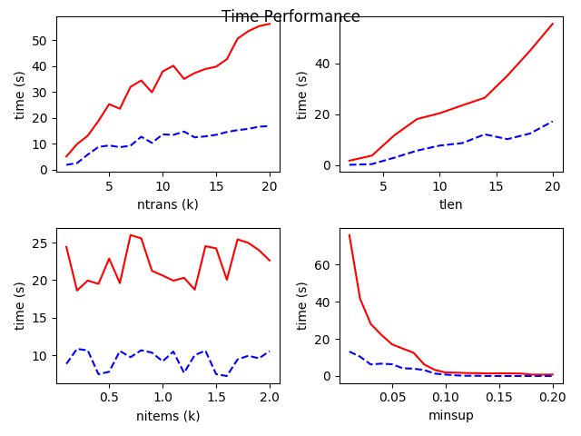
The figures indicate that:
- Basically, FP Growth algorithm is better than Apriori algorithm at most time. It is because FP Growth pre-construct a FP Tree data structure to store the item more “tightly”, which facilitate mining.
- With number of transactions(
ntrans) increasing, both Apriori and FP Growth cost more time. But Apriori cost far more time than FP Growth. - The length of transaction(
tlen) behaves just like thentrans. - The variation of the number of items(
nitems) seems impact less on the time performance. - With the minimal support threshold(
minsup) increasing, both algorithms run faster and their performance become alike. It is because Apriori is able to prune most of candidate itemsets at each step and converges quickly. So, if we want a shorter running time, just make this parameter smaller.
Space/Memory Performance
Notice that:
- The red full line represents Apriori, the blue dash line represents FP Growth.
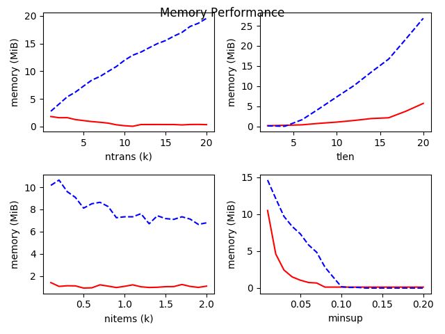
The figures indicate that:
- Basically, the FP Growth takes more memory than Apriori. It is because of not only the pre-construction of FP Tree, but also the recursive construction of conditional FP Tree (the mining procedure).
- With the number of transactions(
ntrans) increasing, FP Growth’s memory consumption increases linearly. But Apriori’s memory consumption stays steady. - With the length of transaction(
tlen) increasing, both Apriori and FP Growth consume more memory. - The variation of the number of items(
nitems) seems impact less on the memory performance. - With the minimal support threshold(
minsup) increasing, both algorithms consume less memory and their performance become alike.
Detailed Time Analysis
(d) Test the running time taken by each major procedure of the algorithms, for example, candidate generation, candidate pruning, and support counting of the Apriori algorithm.
In this Chapter we still use the powerful tool line_profiler to analyze the running time taken by each major procedure of the algorithms. The content of log files are shown in 3.1 Tools & Evaluation Metrics so we won’t explain again.
Since different parameters result in different performance, we randomly sample several of them to analyze.
Notice that:
- the absolute value of time may be meaningless due to the different parameters. We should take focus on their proportion (%) in the whole run time of algorithm.
- The whole run time of the algorithm doesn’t include the time to pre-process the dataset.
Apriori
There are three major procedures in Apriori, “support counting”, “candidate generation” and “candidate pruning”.
Notice that:
- “support counting” is part of “candidate pruning”.
| parameters | support counting (μs) | % | candidate generation (μs) | % | candidate pruning (μs) | % |
|---|---|---|---|---|---|---|
| 1k, 10, 1k, 0.05 | 3868041 | 81.50 | 868597 | 18.30 | 3877056 | 81.68 |
| 5k, 10, 1k, 0.05 | 23639936 | 94.46 | 1376908 | 5.50 | 23649498 | 94.49 |
| 5k, 20, 1k, 0.05 | 45091836 | 91.55 | 4144611 | 8.41 | 45108920 | 91.58 |
| 5k, 10, 0.1k, 0.05 | 24750085 | 93.99 | 1557087 | 5.91 | 24775948 | 94.08 |
| 5k, 10, 1k, 0.20 | 786266 | 71.57 | 311974 | 28.40 | 786564 | 71.60 |
The table above indicates that:
- “Support counting” takes nearly almost all time in the “candidate pruning”. Because each time the Apriori does the pruning operation, it need to scan the whole transaction database and count the support of the itemsets.
- In most cases, “candidate pruning” takes far more time than “candidate generation”.
FP Growth
There are three major procedures in FP Growth, “create tree”, “find prefix path” and “mine tree”.
Notice that:
- “create tree” means creating the first and complete FP Tree, not conditional FP Tree, which is part of “mine tree”.
- “find prefix” is part of “mine tree”.
| parameters | create tree (μs) | % | find prefix path (μs) | % | mine tree (μs) | % |
|---|---|---|---|---|---|---|
| 1k, 10, 1k, 0.05 | 215754 | 11.93 | 123851 | 6.85 | 1593375 | 88.07 |
| 5k, 10, 1k, 0.05 | 3185766 | 25.52 | 409409 | 3.28 | 9299374 | 74.48 |
| 5k, 20, 1k, 0.05 | 14591858 | 44.46 | 1242425 | 3.78 | 18226332 | 55.54 |
| 5k, 10, 0.1k, 0.05 | 6988338 | 41.62 | 540334 | 3.22 | 9802346 | 58.38 |
| 5k, 10, 1k, 0.20 | 252681 | 96.99 | 182 | 0.07 | 7829 | 3.01 |
The table above indicates that:
- FP Growth takes a long time (usually 10%-50%) to build a FP Tree before mining, which helps it save more time in the mining procedure.
- When
minsupis large, building a FP Tree, in fact, is not necessary. Due to this, the Apriori performs well in this situation.
Reference
- Machine Learning in Action, Peter Harrington
- Notice that the code in Chapter 12 Efficiently finding frequent itemsets with FP-growth has some bugs, which make the tree built incorrectly.